Load R Packages
library(tidyverse)    # Data wrangling
library(TwoSampleMR)  # MR
library(gt)
library(RadialMR)     # Radial MR sensetivity analysis
library(phenoscanner)
library(reactable)library(tidyverse) # Data wrangling
library(TwoSampleMR) # MR
library(gt)
library(RadialMR) # Radial MR sensetivity analysis
library(phenoscanner)
library(reactable)R, RadialMR
Radial MR: Produces radial plots and performs radial regression for inverse variance weighted and MR-Egger regression models. These plots have the advantage of improving the visual detection of outliers, as well as being coding invariant. The contribution of each individule SNP to the Cochran’s Q statistic is quantified, with SNPs that have a large contribution been classified as outliers based on significance level selected by the user - typically a bonferonni correction. Outliers can be removed for downstream analysis.
The RadialMR package requires a different input data format to that of TwoSampleMR, so we first use TwoSampleMR::dat_to_RadialMR() to convert our TwoSampleMR harmonized data to the formate required by RadialMR.
# Format data
radial_dat <- mr_dat %>% filter(mr_keep == T) %>% dat_to_RadialMR()
rmr_dat <- radial_dat$TC.AD

# Run Radial MR
bonff = 0.05/nrow(rmr_dat) # Bonferonni Correction
radial_ivw_res <- ivw_radial(rmr_dat, alpha = bonff)
Radial IVW

                  Estimate  Std.Error   t value     Pr(>|t|)
Effect (Mod.2nd) 0.3140916 0.11586058  2.710944 6.709190e-03
Iterative        0.3140955 0.11586121  2.710964 6.708800e-03
Exact (FE)       0.3524370 0.03503782 10.058760 8.405058e-24
Exact (RE)       0.3179997 0.20118635  1.580622 1.177679e-01


Residual standard error: 3.31 on 83 degrees of freedom

F-statistic: 7.35 on 1 and 83 DF, p-value: 0.00815
Q-Statistic for heterogeneity: 909.3152 on 83 DF , p-value: 3.196198e-139

 Outliers detected
Number of iterations = 3radial_egger_res <- egger_radial(rmr_dat, alpha = bonff)
Radial MR-Egger

              Estimate Std. Error   t value    Pr(>|t|)
(Intercept) -0.9612088  0.6654372 -1.444477 0.152415150
Wj           0.5755524  0.2154432  2.671482 0.009106335

Residual standard error: 3.25 on 82 degrees of freedom

F-statistic: 7.14 on 1 and 82 DF, p-value: 0.00911
Q-Statistic for heterogeneity: 866.2584 on 82 DF , p-value: 1.007391e-130

 Outliers detected
As with our core MR methods, we observed that the Radial-MR causal estimates indicated that total cholesteroal is causaly associated with an increased risk of AD, however, there is significant heterogenity.
| b | se | statistic | p | |
|---|---|---|---|---|
| IVW | ||||
| Effect (Mod.2nd) | 0.31 | 0.12 | 2.71 | 0.007 |
| Iterative | 0.31 | 0.12 | 2.71 | 0.007 |
| Exact (FE) | 0.35 | 0.04 | 10.06 | 8.4 × 10⁻²⁴ |
| Exact (RE) | 0.32 | 0.20 | 1.58 | 0.118 |
| Q-Statistic | NA | NA | 909.32 | 3.2 × 10−139 |
| Egger | ||||
| (Intercept) | −0.96 | 0.67 | −1.44 | 0.152 |
| Wj | 0.58 | 0.22 | 2.67 | 0.009 |
| Q-Statistic | NA | NA | 866.26 | 1.0 × 10−130 |
Examining the Radial Plots we also further observe a number of variants were classifed as outliers, which are determined with respect to their contribution to global heterogeneity as quantified by Cochran’s Q-statistic and using a a bonferonni corrected significance threshold.
ivw_radial_p <- plot_radial(radial_ivw_res, radial_scale = F, show_outliers = F)
egger_radial_p <- plot_radial(radial_egger_res, radial_scale = F, show_outliers = F)

cowplot::plot_grid(
  ivw_radial_p + coord_fixed(ratio=0.25) + theme(legend.position = 'bottom'),
   egger_radial_p + theme(legend.position = 'bottom'),
  align = 'h'
)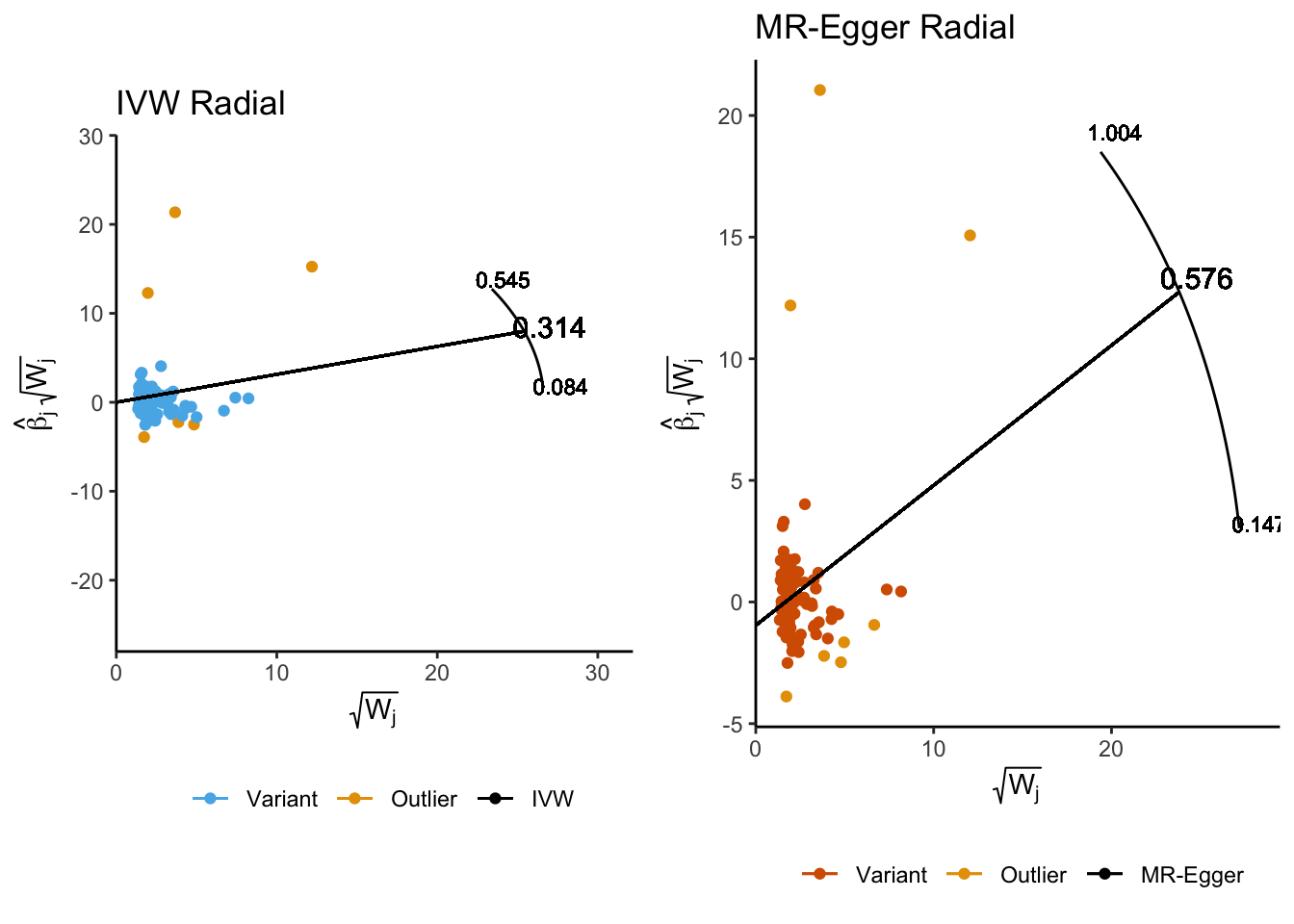
The IVW Radial MR method identified six variants as potential outliers. We can query PhenoScanner to obtain further information on these SNPs (and variants they are in LD with) including what other traits they have been associated with.
# Phenoscanner
phewas_dat <- phenoscanner(
  snpquery=radial_ivw_res$outliers$SNP,
  proxies='EUR',
  r2 = 0.8
  )
PhenoScanner V2
Cardiovascular Epidemiology Unit
University of Cambridge
Email: phenoscanner@gmail.com
Information: Each user can query a maximum of 10,000 SNPs (in batches of 100), 1,000 genes (in batches of 10) or 1,000 regions (in batches of 10) per hour. For large batch queries, please ask to download the data from www.phenoscanner.medschl.cam.ac.uk/data.
Terms of use: Please refer to the terms of use when using PhenoScanner V2 (www.phenoscanner.medschl.cam.ac.uk/about). If you use the results from PhenoScanner in a publication or presentation, please cite all of the relevant references of the data used and the PhenoScanner publications: www.phenoscanner.medschl.cam.ac.uk/about/#citation.
[1] "1 -- chunk of 10 SNPs queried"radial_ivw_res$outliers %>%
left_join(filter(phewas_dat$snps, snp == rsid), by = c("SNP" = "snp")) %>%
select(SNP, Q_statistic, p.value, hg19_coordinates, a1, a2, hgnc) %>%
reactable()Examining the PheWAS results, we can see that three of the outliers (rs7412, rs7568769, and rs8103315) are all located within the APOE region and associated with Alzheimer’s disease. These are the same variants that were previously observed to be driving the IVW causal estimates from the Leave-one-out anlaysis.
Now that have identified outliers, we can re-run our core MR methods with outliers removed. We join the radial MR results to our harmonized dataset and modify the mr_keep variable to flag outliers for removal.
## Modify the mrkeep variable to flag variants as outliers from radial MR for removal
mr_dat_outlier <- mr_dat %>%
  left_join(radial_ivw_res$dat) %>%
  mutate(
     mr_keep = case_when(
       Outliers == "Outlier" ~ FALSE,
       TRUE ~ mr_keep
     )
  )
After removing outliers, the IVW estimates are no longer significant.
# Standard MR
mr_res <- mr(mr_dat, method_list = c(
  c("mr_ivw_fe", "mr_egger_regression", "mr_weighted_median", "mr_weighted_mode")
  ))

## MR analysis
mr_res_outlier <- mr(mr_dat_outlier, method_list = c("mr_ivw_fe", "mr_egger_regression", "mr_weighted_median", "mr_weighted_mode"))

# Heterogeneity statistics
mr_het_outlier <- mr_heterogeneity(mr_dat_outlier, method_list = c("mr_egger_regression", "mr_ivw"))

# Horizontal pleitropy
mr_plt_outlier <- mr_pleiotropy_test(mr_dat_outlier)

# Radial MR
radial_dat_outlier <- mr_dat_outlier %>% filter(mr_keep == T) %>% dat_to_RadialMR()
radial_res_outlier <- ivw_radial(radial_dat_outlier$TC.AD, alpha = 0.05/nrow(radial_dat_outlier$TC.AD))
Radial IVW

                     Estimate  Std.Error    t value  Pr(>|t|)
Effect (Mod.2nd) -0.007293342 0.05138246 -0.1419423 0.8871256
Iterative        -0.007293342 0.05138246 -0.1419423 0.8871256
Exact (FE)       -0.007407696 0.04038259 -0.1834379 0.8544545
Exact (RE)       -0.007357159 0.04651487 -0.1581679 0.8747386


Residual standard error: 1.272 on 77 degrees of freedom

F-statistic: 0.02 on 1 and 77 DF, p-value: 0.887
Q-Statistic for heterogeneity: 124.6615 on 77 DF , p-value: 0.0004808313

 Outliers detected
Number of iterations = 2bind_rows(
mr_res %>% mutate(model = "w/ Outliers"),
mr_res_outlier %>% mutate(model = "w/o Outliers")) %>%
select(model, method, nsnp, b, se, pval) %>%
gt(
groupname_col = "model"
) %>%
fmt_number(
columns = c("b", "se")
) %>%
fmt_number(
columns = pval,
rows = pval > 0.001,
decimals = 3
) %>%
fmt_scientific(
columns = pval,
rows = pval <= 0.001,
decimals = 1
) | method | nsnp | b | se | pval |
|---|---|---|---|---|
| w/ Outliers | ||||
| Inverse variance weighted (fixed effects) | 84 | 0.31 | 0.03 | 1.7 × 10⁻¹⁹ |
| MR Egger | 84 | 0.67 | 0.19 | 7.1 × 10⁻⁴ |
| Weighted median | 84 | 0.05 | 0.07 | 0.434 |
| Weighted mode | 84 | −0.05 | 0.07 | 0.490 |
| w/o Outliers | ||||
| Inverse variance weighted (fixed effects) | 78 | −0.01 | 0.04 | 0.857 |
| MR Egger | 78 | −0.15 | 0.10 | 0.131 |
| Weighted median | 78 | −0.02 | 0.06 | 0.776 |
| Weighted mode | 78 | −0.03 | 0.07 | 0.631 |
This is even more apparant when inspect the scatter and radial plots before and after outlier removal.
# Plots
scatter_p <- mr_scatter_plot(mr_res, mr_dat)
scatter_out_p <- scatter_p[[1]] + theme_bw() +
  guides(color=guide_legend(nrow =1)) +
  labs(title = "w/ outliers") +
  theme(
    text = element_text(size = 8),
    legend.position = 'bottom'
  )

scatter_outlier_p <- mr_scatter_plot(mr_res_outlier, mr_dat_outlier)

scatter_outlier_out_p <- scatter_outlier_p[[1]] + theme_bw() +
  guides(color=guide_legend(nrow =1)) +
  labs(title = "w/o outliers") +
  theme(
    text = element_text(size = 8),
    legend.position = 'bottom'
  )

radial_outlier_p <- plot_radial(radial_res_outlier, radial_scale = F, show_outliers = F)

cowplot::plot_grid(
  scatter_out_p + theme(legend.position = 'none'),
  scatter_outlier_out_p + theme(legend.position = 'none'),
  ivw_radial_p + coord_fixed(ratio=0.25) + theme(legend.position = 'none') + labs(title = "w/ outliers"),
  radial_outlier_p + coord_fixed(ratio=0.2) + theme(legend.position = 'none') + labs(title = "w/o outliers")
)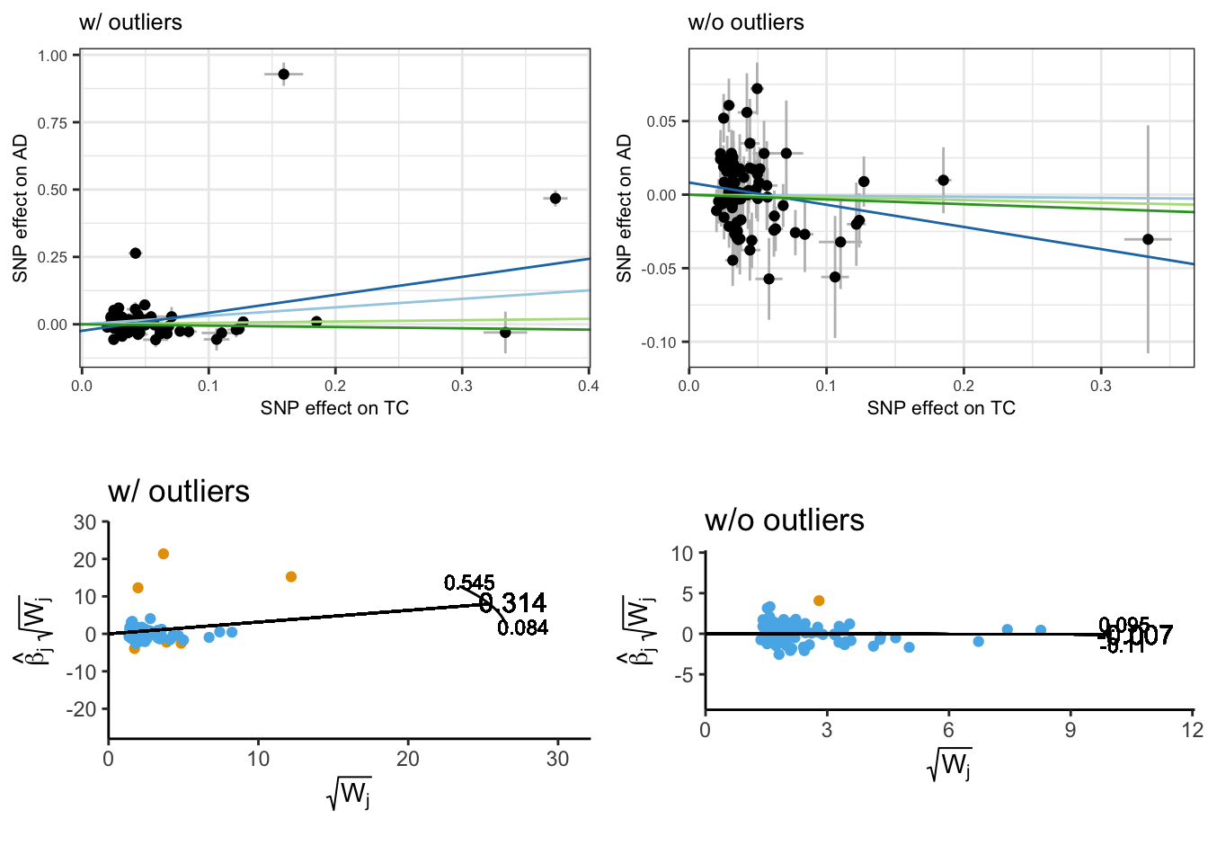
In the initial analysis, six SNPs were identified as potential outliers by Radial-MR. Three of these SNPs were located in the APOE region, known for its large effect size and pleiotropic nature, and were clear outliers based on their Q-statistics. In contrast the other three variants were located elsewhere on the genome and had significanlty smaller Q-statistics. It is possible that the large contribution of the individules APOE variants to the global heterogenity statistcs could be biasing the Q-statistics of other variants.
mr_dat_wo_apoe <- mr_dat %>%
 mutate(
   apoe_region = case_when(
     chr.outcome == 19 & between(pos.outcome, 44912079, 45912079) ~ TRUE,
     TRUE ~ FALSE
   ),
   gws.outcome = ifelse(pval.outcome < 5e-8, TRUE, FALSE),
   mr_keep = case_when(
       apoe_region == TRUE ~ FALSE,
       gws.outcome == TRUE ~ FALSE,
       TRUE ~ mr_keep
     )
 )

# Radial MR
radial_dat_wo_apoe <- mr_dat_wo_apoe %>% filter(mr_keep == T) %>% dat_to_RadialMR()
radial_res_wo_apoe <- ivw_radial(radial_dat_wo_apoe$TC.AD, alpha = 0.05/nrow(radial_dat_wo_apoe$TC.AD))
Radial IVW

                    Estimate  Std.Error    t value  Pr(>|t|)
Effect (Mod.2nd) -0.04916017 0.05347782 -0.9192629 0.3579581
Iterative        -0.04916017 0.05347782 -0.9192629 0.3579581
Exact (FE)       -0.04997953 0.03907883 -1.2789412 0.2009178
Exact (RE)       -0.04961546 0.05031630 -0.9860712 0.3270712


Residual standard error: 1.368 on 80 degrees of freedom

F-statistic: 0.85 on 1 and 80 DF, p-value: 0.361
Q-Statistic for heterogeneity: 149.8155 on 80 DF , p-value: 3.737286e-06

 Outliers detected
Number of iterations = 2radial_wo_apoe_p <- plot_radial(radial_res_wo_apoe, radial_scale = F, show_outliers = F)When the APOE region was removed before conducting radial MR, only two SNPs were now flagged as outliers. These were rs6504872, which was still considered an outlier after removing the APOE region, and a new variant, rs9391858, which emerged as an outlier after this step. This suggests that including the APOE region can bias the Q-statistics of other variants.
cowplot::plot_grid(
  ivw_radial_p + coord_fixed(ratio=0.25) + theme(legend.position = 'none') + labs(title = "w/ APOE"),
  radial_wo_apoe_p + coord_fixed(ratio=0.2) + theme(legend.position = 'none') + labs(title = "w/o APOE"),
  align = 'h'
)
Radial-MR provides an improved visual interpretion of MR analyses and displayes data points with large contributions to Cochran’s Q statistic that are likely to be outliers. Based on this statistical criterion, indivdual variants can be removed from downstream MR analyses to obtain more robust causal estitmates. However, care should be taken when adopting a strategy of removing all outliers until little or no heterogeneity remains. This is highlighted when considering the APOE region, which caused additional variants to be classifed as outliers despite haveing moderate Q-statistics. Exclusion of a particular SNPs should additionaly be based on whether the SNP is associated with separate phenotypes that represent a pleiotropic pathways to the outcome.