7 Multivariable MR

Load R Packages

library(tidyverse)    # Data wrangling 
library(cowplot)
library(TwoSampleMR)  # MR 
library(LDlinkR)      # LD and proxy snps
library(RadialMR)     # Radial MR sensetivity analysis 
library(phenoscanner) # Phenoscaner
library(MVMR)         # Multivarble MR
library(RMVMR)
library(gt)

Import Data

# Define column types for summary statistics
coltypes = cols(
  ID = col_character(),
  CHROM = col_double(),
  POS = col_double(),
  REF = col_character(),
  ALT = col_character(),
  AF = col_double(),
  TRAIT = col_character(),
  BETA = col_double(),
  SE = col_double(),
  Z = col_double(),
  P = col_double(),
  N = col_double(),
  OR = col_double(),
  OR_L95 = col_double(),
  OR_U95 = col_double(),
  DIR = col_character(),
  G1000_ID = col_character(),
  G1000_VARIANT = col_character(),
  DBSNP_ID = col_character(),
  DBSNP_VARIANT = col_character(),
  OLD_ID = col_character(),
  OLD_VARIANT = col_character()
)

## Function for extracting proxy snps using LDLink
munge_proxies <- function(LDLink_file, outcome, outcome_clump){
  LDLink_file_path <- LDLink_file
  proxy_snps <- read_tsv(LDLink_file_path, skip = 1, col_names = F) %>%
    rename(id = X1, func = X2, proxy_snp = X3, coord = X4, alleles = X5, maf = X6, 
           distance = X7, dprime = X8, rsq = X9, correlated_alleles = X10, FORGEdb = X11, RegulomeDB = X12) %>%
    separate(coord, c('chr', 'pos'), sep = ":") %>%
    mutate(snp = ifelse(id == 1, proxy_snp, NA), 
           chr = str_replace(chr, 'chr', ""), 
           chr = as.numeric(chr), 
           pos = as.numeric(pos)) %>%
    fill(snp, .direction = 'down') %>%
    relocate(snp, .before = proxy_snp) %>%
    dplyr::select(-id, -func, -FORGEdb, -RegulomeDB) %>%
    filter(rsq >= 0.8)

  # Munge proxy snp and outcome data
  proxy_outcome <- left_join(
      proxy_snps, outcome, by = c("proxy_snp" = "SNP")
    ) %>%
      separate(correlated_alleles, c("target_a1.outcome", "proxy_a1.outcome", 
                                     "target_a2.outcome", "proxy_a2.outcome"), sep = ",|=") %>%
      filter(!is.na(chr.outcome)) %>%
      arrange(snp, -rsq, abs(distance)) %>%
      group_by(snp) %>%
      slice(1) %>%
      ungroup() %>%
      mutate(
         proxy.outcome = TRUE,
         target_snp.outcome = snp,
         proxy_snp.outcome = proxy_snp, 
      ) %>% 
      mutate(
           new_effect_allele.outcome = case_when(
            proxy_a1.outcome == effect_allele.outcome & proxy_a2.outcome == other_allele.outcome ~ target_a1.outcome,
            proxy_a2.outcome == effect_allele.outcome & proxy_a1.outcome == other_allele.outcome ~ target_a2.outcome,
            TRUE ~ NA_character_
         ), 
          new_other_allele.outcome = case_when(
            proxy_a1.outcome == effect_allele.outcome & proxy_a2.outcome == other_allele.outcome ~ target_a2.outcome,
            proxy_a2.outcome == effect_allele.outcome & proxy_a1.outcome == other_allele.outcome ~ target_a1.outcome,
            TRUE ~ NA_character_
         ), 
         effect_allele.outcome = new_effect_allele.outcome, 
         other_allele.outcome = new_other_allele.outcome
      ) %>%
      dplyr::select(-proxy_snp, -chr, -pos, -alleles, -maf, -distance, -rsq, -dprime,  
             -new_effect_allele.outcome, -new_other_allele.outcome) %>%
      relocate(target_a1.outcome, proxy_a1.outcome, target_a2.outcome, proxy_a2.outcome, .after = proxy_snp.outcome) %>%
      rename(SNP = snp) %>%
      relocate(SNP, .after = samplesize.outcome)
  
  # Merge outcome and proxy outcomes
  outcome_dat <- bind_rows(
    outcome_clump, proxy_outcome
  ) %>% 
    arrange(chr.outcome, pos.outcome)
  
  outcome_dat
}

Methods

Tools & Publications

R, MVMR, RMVMR, TwoSampleMR, MendelianRandomization

Hemani, G. et al. The MR-Base platform supports systematic causal inference across the human phenome. Elife 7, e34408 (2018)
Yavorska, O. O. & Burgess, S. MendelianRandomization: an R package for performing Mendelian randomization analyses using summarized data. Int J Epidemiol 46, dyx034 (2017).
Sanderson, E., Spiller, W. & Bowden, J. Testing and correcting for weak and pleiotropic instruments in two‐sample multivariable Mendelian randomization. Stat Med 40, 5434–5452 (2021).
Woolf, B., Gill, D., Grant, A. J. & Burgess, S. MVMRmode: Introducing an R package for plurality valid estimators for multivariable Mendelian randomisation. medRxiv (2023).

Multivariable MR: Used to estimate the causal relationships between multiple exposures and a single outcome. It is particularly useful in situations where multiple exposures are related and have potential inter-related effects on the outcome of interest. MVMR can help to disentangle the complex relationships between these exposures and provide insights into their independent causal effects. Examples of situations where MVMR can be useful include the estimation of the independent effects of related risk factors such as lipid fractions on an outcome, or the assessment of the independent effects of a primary risk factor and a secondary mediator on a disease outcome.

Harmonizing SumStats for MVMR

MVMR involves the simultaneous use of multiple exposures as instrumental variables in the analysis of a single outcome. As such, harmonizing the exposure and outcome datasets for MVMR is a more complex process than in univariable MR as it requires conducting multiple clumping and proxy-variant procedures. The following is a step-by-step guide to harmonizing the exposure and outcome datasets for MVMR using LDL and HDL cholesterol levels as the exposures, and AD as the outcome.

Import datasets

Import LDL SumStats

exposure1_path = "resources/Willer2013ldl.chrall.CPRA_b37.tsv.gz"
exposure1_ss <- read_tsv(exposure1_path, comment = "##", col_types = coltypes, 
                       col_select = c(DBSNP_ID, CHROM, POS, REF, ALT, AF, BETA, SE, Z, P, N, TRAIT))

# Format data to TwoSampleMR format
exposure1 <- exposure1_ss %>%
  format_data(.,
    type = "exposure",
    snps = NULL,
    header = TRUE,
    phenotype_col = "TRAIT",
    snp_col = "DBSNP_ID",
    beta_col = "BETA",
    se_col = "SE",
    eaf_col = "AF",
    effect_allele_col = "ALT",
    other_allele_col = "REF",
    pval_col = "P",
    samplesize_col = "N",
    z_col = "Z",
    chr_col = "CHROM",
    pos_col = "POS",
    log_pval = FALSE
) %>%
  as_tibble()

Import HDL SumStats

exposure2_path = "resources/Willer2013hdl.chrall.CPRA_b37.tsv.gz"
exposure2_ss <- read_tsv(exposure2_path, comment = "##", col_types = coltypes, 
                       col_select = c(DBSNP_ID, CHROM, POS, REF, ALT, AF, BETA, SE, Z, P, N, TRAIT))

# Format data to TwoSampleMR format
exposure2 <- exposure2_ss %>%
  format_data(.,
    type = "exposure",
    snps = NULL,
    header = TRUE,
    phenotype_col = "TRAIT",
    snp_col = "DBSNP_ID",
    beta_col = "BETA",
    se_col = "SE",
    eaf_col = "AF",
    effect_allele_col = "ALT",
    other_allele_col = "REF",
    pval_col = "P",
    samplesize_col = "N",
    z_col = "Z",
    chr_col = "CHROM",
    pos_col = "POS",
    log_pval = FALSE
) %>%
  as_tibble()

Import AD SumStats

outcome_path = "resources/Kunkle2019load_stage123.chrall.CPRA_b37.tsv.gz"
outcome_ss <- read_tsv(outcome_path, comment = "##",  col_types = coltypes, 
                       col_select = c(DBSNP_ID, CHROM, POS, REF, ALT, AF, BETA, SE, Z, P, N, TRAIT))

# Format outcome
outcome <- outcome_ss %>%
  format_data(.,
    type = "outcome",
    snps = NULL,
    header = TRUE,
    phenotype_col = "TRAIT",
    snp_col = "DBSNP_ID",
    beta_col = "BETA",
    se_col = "SE",
    eaf_col = "AF",
    effect_allele_col = "ALT",
    other_allele_col = "REF",
    pval_col = "P",
    samplesize_col = "N",
    z_col = "Z",
    chr_col = "CHROM",
    pos_col = "POS",
    log_pval = FALSE
) %>%
  as_tibble()

Exposures

Clump Exposure datasets

# Clump ldl
exposure1_clump <- exposure1 %>% 
  filter(pval.exposure < 0.01) %>%
  clump_data(.,
  clump_kb = 10000,
  clump_r2 = 0.001,
  clump_p1 = 1,
  clump_p2 = 1,
  pop = "EUR"
)

exposure1_dat <- filter(exposure1_clump, pval.exposure < 5e-8)

# Clump HDL
exposure2_clump <- exposure2 %>% 
  filter(pval.exposure < 0.01) %>%
  clump_data(.,
  clump_kb = 10000,
  clump_r2 = 0.001,
  clump_p1 = 1,
  clump_p2 = 1,
  pop = "EUR"
)

exposure2_dat <- filter(exposure2_clump, pval.exposure < 5e-8)

Perform clumping to obtain independent genome-wide significant variants for each exposure. This step involves identifying the SNPs that are independently associated with each exposure and are significant at the genome-wide level.

There are 79 and 89 independent genome-wide significant SNPS for LDL and HDL respectivly.

Combine Exposures

## Make list of distinct SNPs from the exposures independent GWS snps 
mvmr_snps <- bind_rows(
  select(exposure1_dat, SNP), 
  select(exposure2_dat, SNP), 
) %>%
  distinct(SNP) %>%
  pull(SNP)

## extract combined SNP list from exposure datasets 
comb_exp <- bind_rows(
  exposure1 %>% filter(SNP %in% mvmr_snps),
  exposure2 %>% filter(SNP %in% mvmr_snps),
)

Combine the exposure SNP lists and extract all the SNPs from each exposure. This step combines the lists of SNPs for each exposure and extracts all the SNPs that are present in each exposure.

Combine Exposures

## Unique SNP ids across exposures
exp_snp_list <- full_join(
  select(exposure1_dat, SNP, exposure), 
  select(exposure2_dat, SNP, exposure), 
  by = 'SNP'
)

exp1_unq_snps <- filter(exp_snp_list, !is.na(exposure.x) & is.na(exposure.y)) %>% nrow()
exp2_unq_snps <- filter(exp_snp_list, !is.na(exposure.y) & is.na(exposure.x)) %>% nrow()
both_unq_snps <- filter(exp_snp_list, !is.na(exposure.y) & !is.na(exposure.x)) %>% nrow()

There are 164 unique SNPs across the LDL and HDL SNP list - 75 unique to LDL, 85 to HDL, and 4 that are shared.

Extracting these 164 SNPs from the LDL and HDL SumStats we get the following count of genome-wide significant SNPs across both traits.

Combined Exposure SNPs

## exposure and outcome snps lists 
comb_exp_out <- bind_rows(
  exposure1 %>% filter(SNP %in% mvmr_snps) %>% 
    rename(pval = pval.exposure, trait = exposure, chr = chr.exposure, pos = pos.exposure), 
  exposure2 %>% filter(SNP %in% mvmr_snps) %>% 
    rename(pval = pval.exposure, trait = exposure, chr = chr.exposure, pos = pos.exposure), 
  outcome %>% filter(SNP %in% mvmr_snps) %>% 
    rename(pval = pval.outcome, trait = outcome, chr = chr.outcome, pos = pos.outcome)
)

## How many SNPs are GWS across the exposures 
comb_exp_wide <- comb_exp_out %>%
   arrange(chr, pos) %>%
   select(SNP, trait, pval) %>%
   pivot_wider(names_from = trait, values_from = pval) %>%
   mutate(pval.exposure = pmin(LDL, HDL, na.rm = T))

comb_exp_wide %>% count(LDL < 5e-8, HDL < 5e-8)  %>%
  gt()

LDL < 5e-08	HDL < 5e-08	n
FALSE	TRUE	76
TRUE	FALSE	64
TRUE	TRUE	24

Identify proxy variants for any SNPs that are missing in each exposure. This step involves identifying proxy variants for any SNPs that are not present in each exposure dataset. This is necessary to ensure that the exposure datasets are complete and that all relevant SNPs are included in the analysis.

Note

There are no missing variants between the LDL &HDL SumStats, as such there is no need identify proxy variants

Perform LD clumping on the combined SNP list to retain indepdent SNPs. This step is performed to reduce the risk of spurious results arising due to multi-collinearity by including correlated SNPs. LD clumping identifies lead SNPs in each locus and discards the remaining SNPs that are in linkage disequilibrium with them.

Clump Combined Exposures

## Do another round of LD clumping 
clump_comb_exp <- comb_exp_wide %>% 
  clump_data(.,
  clump_kb = 10000,
  clump_r2 = 0.001,
  clump_p1 = 1,
  clump_p2 = 1,
  pop = "EUR"
)

comb_exp_independent <- comb_exp %>% filter(SNP %in% clump_comb_exp$SNP)

Due to the high correlation among genetic variants, the GWAS of HDL and LDL may identify loci in the same genomic region. After LD clumping on the smallest p-value from the exposures, we retained 136 of the initial 164 SNPs, ensuring that we included only independent variants in the analysis.

LDL < 5e-08	HDL < 5e-08	n
FALSE	TRUE	66
TRUE	FALSE	57
TRUE	TRUE	13

Outcome

Extract exposures SNPs from the outcome GWAS. This step involves extracting the SNPs that are associated with the exposures from the genome-wide association study of the outcome.

Extract Exposure SNPs from Outcome

# extract exposure SNPs present in outcome
outcome_clump <- semi_join(
  outcome, comb_exp_independent, by = "SNP"
)

# Exposure SNPs not present in outomce
outcome_wo_snps <- anti_join(
  comb_exp_independent, outcome, by = "SNP"
) %>%
  distinct(SNP)

Of the 136 exposures SNPs, 135 are available in the AD SumStats - with 1 variant missing.

Note

One issue to be aware of is that 3 of the exposure SNPs are GWS for AD and are violating the exclusion restriction assumption.

LDL < 5e-08	HDL < 5e-08	AD < 5e-08	n
FALSE	TRUE	FALSE	65
FALSE	TRUE	NA	1
TRUE	FALSE	FALSE	55
TRUE	FALSE	TRUE	2
TRUE	TRUE	FALSE	12
TRUE	TRUE	TRUE	1

Identify proxy variants for any SNPs that missing in the outcome. This step involves identifying proxy variants for any SNPs that are not present in the outcome dataset. This is necessary to ensure that the outcome dataset is complete and that all relevant SNPs are included in the analysis.

Extract proxy SNPs for outcome

# Use LDLinkR to identify proxy snps
LDproxy_batch(outcome_wo_snps, 
        pop = "CEU", 
        r2d = "r2", 
        token = 'a6deee62cc4a', 
        append = TRUE,
        genome_build = "grch37")


Submitting request for query variant rs2729816.
Checking status of server...Combined file for all query variants saved to:
/Users/sheaandrews/gitcode/MR-tutorial/combined_query_snp_list_grch37.txt

Extract proxy SNPs for outcome

system("mv combined_query_snp_list_grch37.txt data/mvmr_proxy_snps.txt")

# Munge proxy snp file
outcome_dat <- munge_proxies("data/mvmr_proxy_snps.txt", outcome, outcome_clump)

Harmonize

Harmonize exposure and outcome datasets. In order to perform MR the effect of a SNP on an outcome and exposure must be harmonised to be relative to the same allele.

Harmonize exposure and outcome datasets

# Univariate MR 
mrdat <- harmonise_data(comb_exp, outcome_dat) %>%
  as_tibble() %>%
  filter(pval.exposure < 5e-8)

## MVMR
mvdat <- mv_harmonise_data(comb_exp, outcome_dat)

Export MVMR datasets

write_csv(mrdat, 'data/harmonized_mvmr_uni.csv')
write_rds(mvdat, 'data/harmonized_mvmr.rds')

MVMR Analysis

TwoSampleMR

Univariable MR

## Univariate MR
mr_res <- mr(mrdat, method_list = c("mr_ivw_fe", "mr_egger_regression", "mr_weighted_median", "mr_weighted_mode"))

# Heterogeneity statistics 
het_res <- mr_heterogeneity(mrdat, method_list = c("mr_egger_regression", "mr_ivw"))

# Horizontal pleitropy
plei_res <- mr_pleiotropy_test(mrdat)

# Leave-one-out analysis 
res_loo <- mr_leaveoneout(mrdat, method = mr_ivw_fe) %>% as_tibble()

# Single SNP anlaysis 
res_single <- mr_singlesnp(mrdat, all_method = c("mr_ivw_fe", "mr_egger_regression", "mr_weighted_median", "mr_weighted_mode")) %>% as_tibble()

# Radial MR 
radial_dat <- mrdat %>% filter(mr_keep == T) %>% dat_to_RadialMR()
radial_res <- map(radial_dat, function(x){
    ivw_radial(x, alpha = 0.05/nrow(x))
  }
)


Radial IVW

                   Estimate  Std.Error   t value     Pr(>|t|)
Effect (Mod.2nd) -0.1223808 0.11024660 -1.110064 0.2669712358
Iterative        -0.1223809 0.11024665 -1.110065 0.2669710759
Exact (FE)       -0.1365797 0.04139487 -3.299436 0.0009687925
Exact (RE)       -0.1242786 0.09937333 -1.250623 0.2149596925


Residual standard error: 2.664 on 75 degrees of freedom

F-statistic: 1.23 on 1 and 75 DF, p-value: 0.271
Q-Statistic for heterogeneity: 532.1109 on 75 DF , p-value: 4.739116e-70

 Outliers detected 
Number of iterations = 3

Radial IVW

                  Estimate Std.Error  t value     Pr(>|t|)
Effect (Mod.2nd) 0.2897672 0.1082519 2.676786 7.433216e-03
Iterative        0.2897684 0.1082525 2.676782 7.433288e-03
Exact (FE)       0.3190728 0.0356857 8.941193 3.849920e-19
Exact (RE)       0.2930763 0.1527847 1.918230 5.934461e-02


Residual standard error: 3.035 on 67 degrees of freedom

F-statistic: 7.17 on 1 and 67 DF, p-value: 0.00934
Q-Statistic for heterogeneity: 617.3408 on 67 DF , p-value: 5.309971e-90

 Outliers detected 
Number of iterations = 3

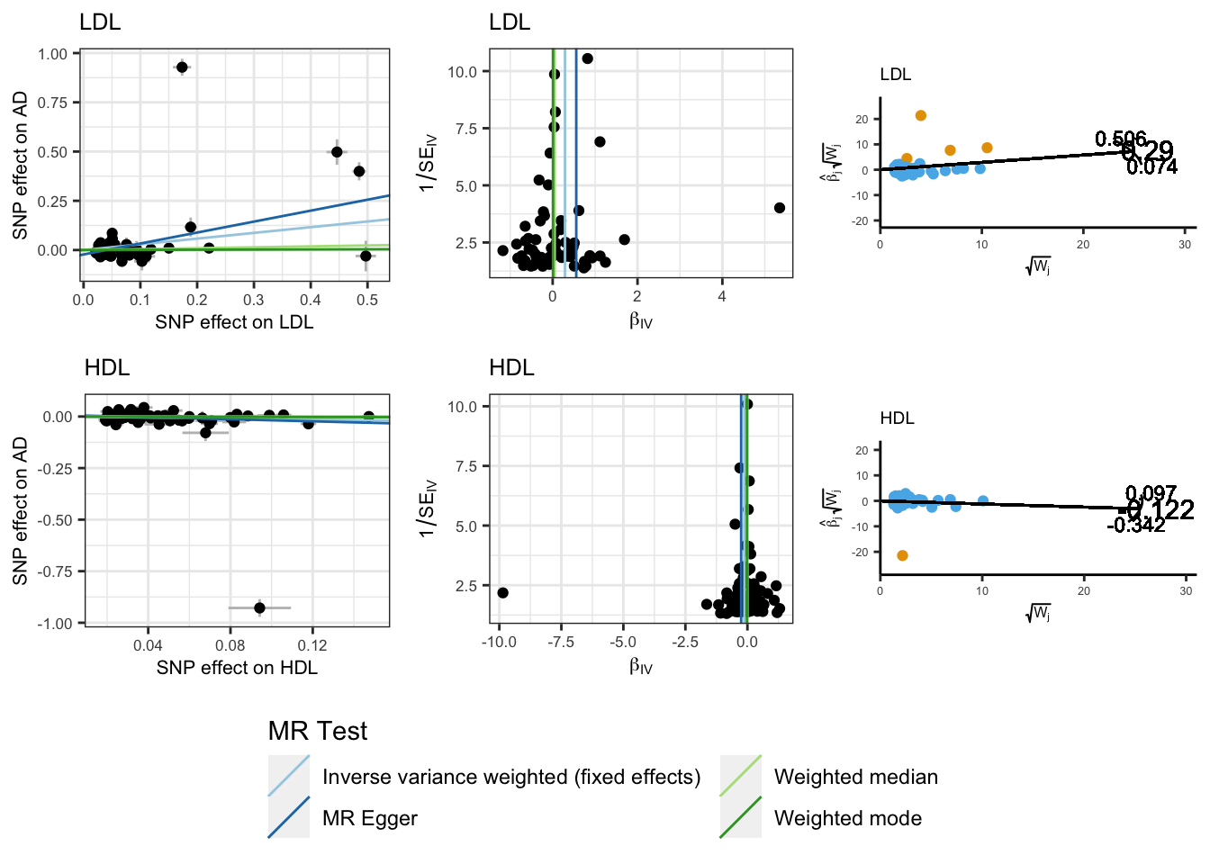
Using the core univariable MR methods, we observe that higher genetically predicted LDL and HDL are associated with increased and reduced risk of AD respectively.

Univariable MR Results
outcome	exposure	method	nsnp	b	se	pval
AD	LDL	Inverse variance weighted (fixed effects)	68	0.29	0.04	3.3 × 10⁻¹⁶
AD	LDL	MR Egger	68	0.56	0.16	6.6 × 10⁻⁴
AD	LDL	Weighted median	68	0.05	0.06	0.451
AD	LDL	Weighted mode	68	0.01	0.06	0.901
AD	HDL	Inverse variance weighted (fixed effects)	76	−0.12	0.04	0.003
AD	HDL	MR Egger	76	−0.25	0.20	0.214
AD	HDL	Weighted median	76	0.00	0.07	0.998
AD	HDL	Weighted mode	76	−0.02	0.07	0.795

However, as with total cholesterol levels we observe significant heterogeneity suggesting that the IVW estimates are likely to be biased.

Heterogenity tests for univariable MR
outcome	exposure	method	Q	Q_df	Q_pval
AD	LDL	MR Egger	576.56	66	1.4 × 10⁻⁸²
AD	LDL	Inverse variance weighted	623.54	67	3.3 × 10⁻⁹¹
AD	HDL	MR Egger	528.75	74	7.5 × 10⁻⁷⁰
AD	HDL	Inverse variance weighted	533.03	75	3.2 × 10⁻⁷⁰

Egger intercept tests for pleiotropy
outcome	exposure	egger_intercept	se	pval
AD	LDL	−0.02	0.01	0.024
AD	HDL	0.01	0.01	0.442

Plots for MR results

scatter_p <- mr_scatter_plot(mr_res, mrdat)

funnel_p <- mr_funnel_plot(res_single)

radial_p <-  map(radial_res, function(x){
     plot_radial(x, radial_scale = F, show_outliers = F)
  }
)

joint_mr_p <- cowplot::plot_grid(
  scatter_p[[1]] + labs(title = "LDL") + theme_bw() + theme(legend.position = 'none', text = element_text(size = 8)),
  funnel_p[[1]] + labs(title = "LDL") + theme_bw() + theme(legend.position = 'none', text = element_text(size = 8)), 
  radial_p[[2]] + labs(title = "LDL") + coord_fixed(ratio=0.25) + theme(legend.position = 'none', text = element_text(size = 6)), 
  scatter_p[[2]] + labs(title = "HDL") + theme_bw() + theme(legend.position = 'none', text = element_text(size = 8)), 
  funnel_p[[2]] + labs(title = "HDL") + theme_bw() + theme(legend.position = 'none', text = element_text(size = 8)),
  radial_p[[1]] + labs(title = "HDL") + coord_fixed(ratio=0.25) + theme(legend.position = 'none', text = element_text(size = 6))
  )


legend_scatter <- cowplot::get_legend(
  # create some space to the left of the legend
  scatter_p[[1]] + theme(legend.box.margin = margin(12, 12, 12, 12))
)

# add the legend to the row we made earlier. Give it one-third of 
# the width of one plot (via rel_widths).
scatter_out.p <- cowplot::plot_grid(joint_mr_p, legend_scatter, rel_heights = c(4, 1), nrow = 2)
scatter_out.p

Extending these analyses into a multivariable framework we are able to determine the independent effects of LDL and HDL cholesterol levels on AD. We observed that higher genetically predicted LDL remains significantly causally associated with increased AD risk, while the causal effect of HDL on AD is now non-significant.

MVMR analysis

mvmr_res <- mv_multiple(mvdat, plots = F)

MVMR Results
exposure	outcome	nsnp	b	se	pval
LDL	AD	68	0.27	0.08	8.7 × 10⁻⁴
HDL	AD	76	−0.12	0.09	0.201

MVMR package

The MVMR R package can be used to perform multivariable Mendelian randomization analyses, which includes heterogeneity statistics to assess the strength and validity of the instruments. Additionally, it can evaluate conditional instrument strength and pleiotropic bias.

Format for MVMR

mvmr_dat <- cbind(mvdat$exposure_beta, 
        mvdat$exposure_se, 
        mvdat$outcome_beta, 
        mvdat$outcome_se
      ) %>%
      as.data.frame() %>%
      rownames_to_column() %>%
      as.matrix()

F.data <- format_mvmr(BXGs = mvmr_dat[,c(2,3)],
                    BYG = mvmr_dat[,6],
                    seBXGs = mvmr_dat[,c(4,5)],
                    seBYG = mvmr_dat[,7],
                    RSID = mvmr_dat[,1])

Results for MVMR

res_mvmr <- ivw_mvmr(r_input = F.data)


Multivariable MR

            Estimate Std. Error   t value    Pr(>|t|)
exposure1  0.2689424 0.08080841  3.328149 0.001135234
exposure2 -0.1202465 0.09404536 -1.278601 0.203298214

Residual standard error: 2.293 on 131 degrees of freedom

Results for MVMR

mvmr_out <- res_mvmr %>% 
    as.data.frame() %>%
    rownames_to_column() %>%
    as_tibble() %>% 
    janitor::clean_names() %>%
    rename(exposure = rowname, b = estimate, se = std_error, p = pr_t) %>%
    mutate(
      exposure = ifelse(exposure == 'exposure1', 'LDL', 'HDL'), 
      outcome = 'AD',
      method = 'IVW-MVMR'
    ) %>%
    relocate(outcome, method, .after = exposure)

MVMR package Results
exposure	outcome	method	b	se	t_value	p
LDL	AD	IVW-MVMR	0.27	0.08	3.33	0.001
HDL	AD	IVW-MVMR	−0.12	0.09	−1.28	0.203

MVMR Diagnostics

sres <- strength_mvmr(r_input = F.data, gencov = 0)


Conditional F-statistics for instrument strength

            exposure1 exposure2
F-statistic  77.75899  70.85811

MVMR Diagnostics

pres <- pleiotropy_mvmr(r_input = F.data, gencov = 0)

Q-Statistic for instrument validity:
681.9149 on 130 DF , p-value: 1.007841e-75

Note

Calculating heterogeneity statistics requires the covariance between the effect of the genetic variants on each exposure to be known. This can either be estimated from individual level data, be assumed to be zero, or fixed at zero using non-overlapping samples of each exposure GWAS.

Here, Q- and F-statistics are estimated assuming a genetic covariance of 0. Phenotypic correlations can calcuated from summary statistics using PhenoSpD.

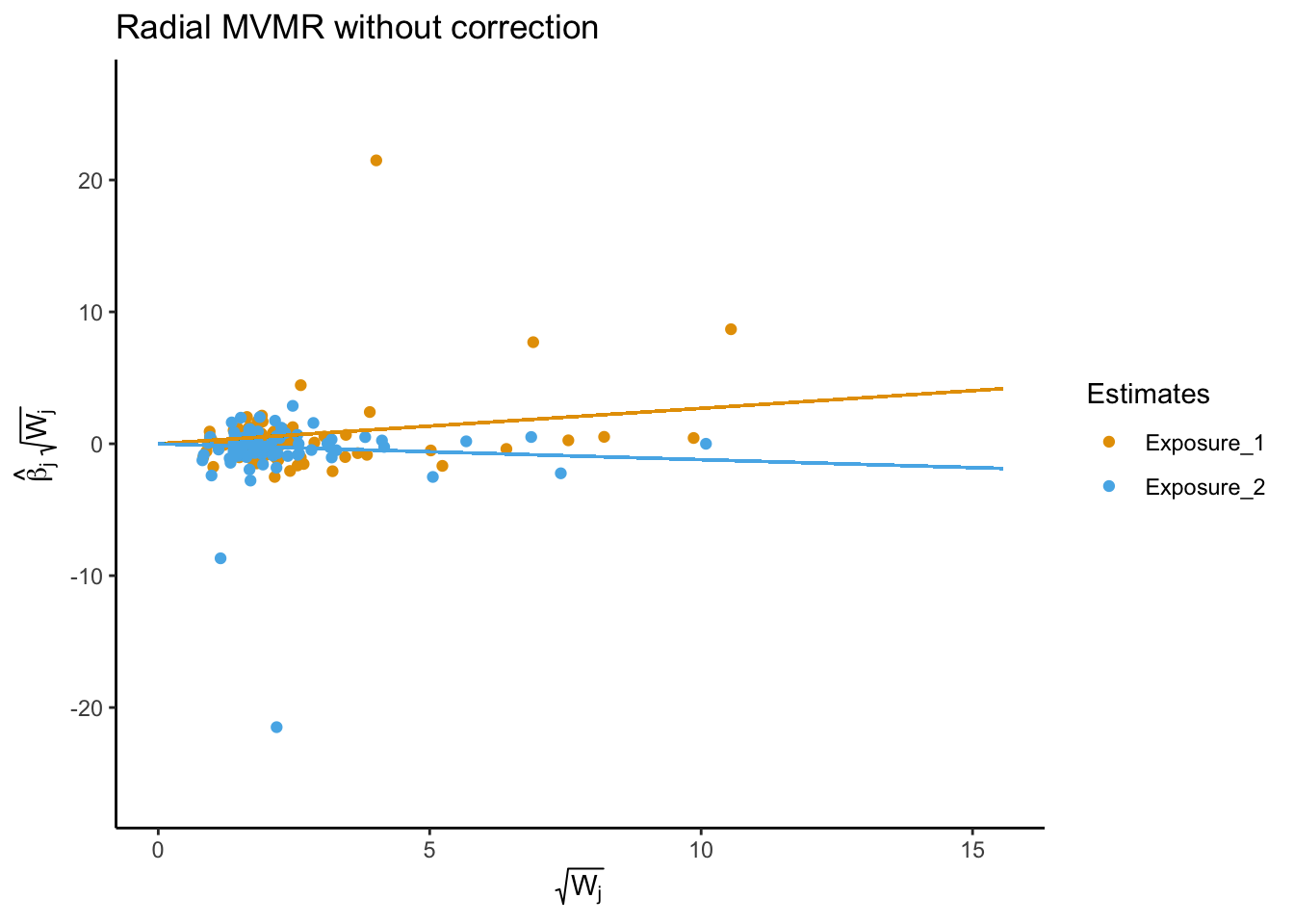
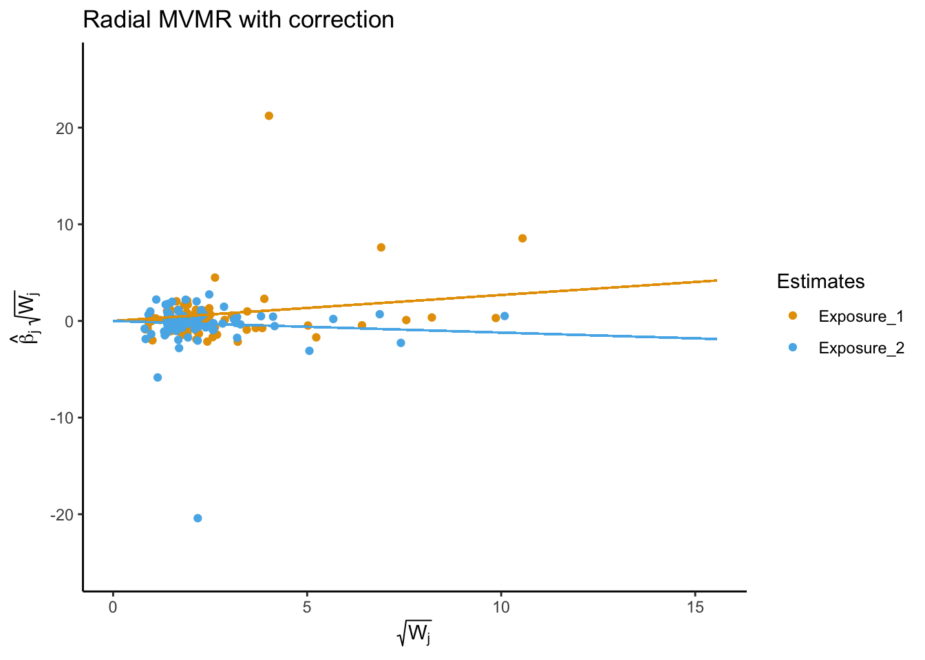
RMVMR

Radial MVMR is an extension of the MVMR package to perform radial multivariable Mendelian randomization analyses, including generating radial-MVMR plots to show the causal effect of each exposure on the outcome.

Results for MVMR

F.data_rmvmr <- format_rmvmr(BXGs = mvmr_dat[,c(2,3)],
                    BYG = mvmr_dat[,6],
                    seBXGs = mvmr_dat[,c(4,5)],
                    seBYG = mvmr_dat[,7],
                    RSID = mvmr_dat[,1])


res_rmvrm <- ivw_rmvmr(F.data_rmvmr)


Radial Multivariable MR

            Estimate Std. Error   t value    Pr(>|t|)
exposure1  0.2689424 0.08080841  3.328149 0.001135234
exposure2 -0.1202465 0.09404536 -1.278601 0.203298214

Residual standard error: 2.293 on 131 degrees of freedom

Results for MVMR

sres_rmvrm <- strength_rmvmr(F.data_rmvmr, gencov = 0)

RMVMR Plot

rmvrm_p <- plot_rmvmr(F.data_rmvmr, res_rmvrm)

rmvrm_p

$p1

$p2


attr(,"class")
[1] "RMVMR_plot"

MendelianRandomization package

The MendelianRandomization package provides additional functions for MVMR versions of MR-Egger and Weighted Median Estimators.

Results for MVMR Sensetivity analyses

MRMVInputObject <- MendelianRandomization::mr_mvinput(
  bx = mvdat$exposure_beta, 
  bxse = mvdat$exposure_se,
  by = mvdat$outcome_beta,
  byse = mvdat$outcome_se,
  snps = rownames(mvdat$exposure_beta), 
  exposure = c('LDL', 'HDL'), 
  outcome = 'AD'
  )

MRMV_ivw <- MendelianRandomization::mr_mvivw(MRMVInputObject, 
                       model="default", 
                       correl=FALSE, 
                       distribution="normal",
                       alpha = 0.05)

MRMV_ivw_df <- cbind(MRMV_ivw@Exposure, MRMV_ivw@Outcome, MRMV_ivw@Estimate, MRMV_ivw@StdError, MRMV_ivw@Pvalue) %>%
  as_tibble() %>%
  magrittr::set_colnames(c("Exposure", "Outcome", "b", "se", "p")) %>%
  mutate(method = "MRMV-IVW")

MRMV_egger <- MendelianRandomization::mr_mvegger(MRMVInputObject, orientate = 1, correl = FALSE, distribution = "normal", alpha = 0.05)

MRMV_egger_df <- cbind(MRMV_egger@Exposure, MRMV_egger@Outcome, MRMV_egger@Estimate, MRMV_egger@StdError.Est, MRMV_egger@Pvalue.Est) %>%
  as_tibble() %>%
  magrittr::set_colnames(c("Exposure", "Outcome", "b", "se", "p")) %>%
  mutate(method = "MRMV-Egger")


MRMV_wme <- MendelianRandomization::mr_mvmedian( MRMVInputObject, distribution = "normal", alpha = 0.05, iterations = 10000, seed = 314159265 )

MRMV_wme_df <- cbind(MRMV_wme@Exposure, MRMV_wme@Outcome, MRMV_wme@Estimate, MRMV_wme@StdError, MRMV_wme@Pvalue) %>%
  as_tibble() %>%
  magrittr::set_colnames(c("Exposure", "Outcome", "b", "se", "p")) %>%
  mutate(method = "MRMV-WME")

MVMR Sensetivity Results
Exposure	Outcome	method	b	se	p
LDL	AD	MRMV-Egger	0.43	0.10	9.8 × 10⁻⁶
HDL	AD	MRMV-Egger	−0.12	0.09	0.174
LDL	AD	MRMV-WME	0.04	0.06	0.544
HDL	AD	MRMV-WME	0.01	0.06	0.911

MVMRmode Package

The MVMRmode pacakge implements a plurality valid sensitivity analysis for multivariable-MR.

Note

This method and corresponding R package are very new, needs further testing.

Results for MVMRmode

MRMV_wbe_res <- MVMRmode::mv_mrmode(Bout = mvdat$outcome_beta, 
                    Bexp = mvdat$exposure_beta, 
                    SEout = mvdat$outcome_se, 
                    SEexp = mvdat$exposure_se, 
                    Psi=0, CIMin = NA, CIMax = NA, CIStep = 0.001, alpha = 0.05, 
                    residual="IVW",Mode="CM",weighting = "weighted", stderror = "simple", 
                    phi = 1,distribution = "normal",iterations = 10000)

MRMV_wbe_df <- as_tibble(MRMV_wbe_res) %>%
  rename(b = Estimate, p = Pvalue) %>%
  mutate(Exposure = c("HDL", "LDL"), 
         Outcome = "AD", 
         method = 'MRMV_WBE') %>%
  mutate_if(is.double, as.character)

MVMR Sensetivity Results
Exposure	Outcome	method	b	CILower	CIUpper	p	NvalidSNPs	Nrange
HDL	AD	MRMV_WBE	−0.03	−0.11	0.05	0.495	117	1
LDL	AD	MRMV_WBE	−0.07	−0.16	0.05	0.151	117	1

Summary

Multivariable MR allows estimation of causal relationships between multiple exposures and a single outcome. In univariable MR, we observed that HDL cholesterol levels are associated with a reduced risk of AD, while LDL cholesterol is associated with an increased risk. However, both exposures are highly correlated, and it is difficult to estimate the independent effects of HDL and LDL cholesterol on AD. Using MVMR, we found that after adjusting for the effects of LDL cholesterol, HDL cholesterol was no longer independently associated with AD. This suggests that the observed association between HDL cholesterol and AD risk in univariable MR analyses may be driven by the shared effects of LDL cholesterol.

Outcome	method	LDL			HDL
Outcome	method	b	se	p	b	se	p
AD	MRMV-IVW	0.27	0.08	8.7 × 10⁻⁴	−0.12	0.09	0.201
AD	MRMV-Egger	0.43	0.10	9.8 × 10⁻⁶	−0.12	0.09	0.174
AD	MRMV-WME	0.04	0.06	0.544	0.01	0.06	0.911
AD	MRMV_WBE	−0.07	NA	0.151	−0.03	NA	0.495